Contour plots are plots that draw a 3-D surface on a 2-D plot. They are characterized by the slices for the z-axis that are called contours. Hence, contour plots answer to the question 'how z is changing as a function of x and y'. They are often being used to plot results from experiments where x and y are two input variables and z is the output of the experiment.
R has many functions for calculating contours and displaying x,y plots. The most common is the contour function. Sometimes a good alternative, the filled.contour function can provide a clear understanding of the transition of z for the given x and y.
Although contour plots are very efficient in displaying the z variable given two input variables, there are cases where an experiment is repeated for different values over a set of values of a third variable. In these cases, there is a need to project the output w given the input values of x, y and z.
A simple solution is to create a series of contour plots, where each contour shows variable w in respect of x and y, for a given value of z (in the case dealt here, we require that z is available at distinct values/levels). Another solution, that has been proposed here, is to create a superimposed image of one standard (line) contourplot with a second one, color-filled. Although this solution addresses the fact that different measurements of w are shown for x, y and z, it is limited to using at maximum two different levels (two values) of z, since more levels reduce the plot clarity. Moreover, in some cases, the resulting plot from that method cannot be interpreted nicely, as it will be seen in the example that follows.
To address these issues, the proposed solution here is the use of a 3D plot where the contour plots are superimposed. In this way, the reader can visualize both the contour levels of each x, y, z input set, and the relative distance of each of the x, y surfaces for different values of z.
The main function presented here, contour4D, uses a persp3d function to initially draw the first surface, and then superimposes the plot with the rest surfaces using the surface3d function. The input is two vectors x and y, and one list of vectors W containing z vectors of the w output for each combination of x and y, given a value/level of z. The last parameter is the vector size of z. The function also handles color adjustment to help distinguishing among the different surfaces.
library(rgl)
library(colorspace)
#---------------------------------------------------------#
# Function: contour4D #
# Version: 1.0.1 #
# Date: 19/07/13 #
# Author: Athanasios Tsakonas #
# Inputs: #
# x, y: vectors of size N,M #
# W: list of size z,containing vectors of size NxM #
# Variables: #
# pal,lpal: palette vectors for surfaces, contour lines#
# clines: contour lines of surfaces #
#---------------------------------------------------------#
contour4D <- function(x, y, W) {
pal<-rainbow_hcl(length(W), start = 90, end = -30)
lpal<-rainbow_hcl(length(W), start = 70, end = -50)
persp3d(x,y,W[[1]], col=pal[1], alpha=0.5, axes=T, zlab='z')
clines <- contourLines(x,y,W[[1]])
for (i in 1:length(clines))
with(clines[[i]], lines3d(x, y, level, col=lpal[1]))
for (k in 2:length(W)) {
surface3d(x,y,W[[k]], col=pal[k], alpha=0.5, axes=F)
clines <- contourLines(x,y,W[[k]])
for (i in 1:length(clines))
with(clines[[i]], lines3d(x, y, level, col=lpal[k]))
}
}
To demonstrate the function output we'll consider an artificial data problem. We first create some data in the required input form.
#declare functions to be used for producing some output;
#each of the functions is assumed to be output for a different z value
f1 <- function(x, y) (x^2 + y^2 + sin(x*y)+ 1.2)
f2 <- function(x, y) (x^2 + y^2 + sin(x*y)+ 0.7)
f3 <- function(x, y) (x^2 + y^2 + sin(x*y)+ 0.2)
#add some jittering to the data, for more realistic results
a1<-rnorm(15*15)
a2<-rnorm(15*15)
a3<-rnorm(15*15)
#generate some x, y
y <- seq(-1,1,len=15)
#now produce output for each of the z levels
w1 <- outer(x, y, f1) + 0.08*a1
w2 <- outer(x, y, f2) + 0.08*a2
w3 <- outer(x, y, f3) + 0.08*a3
#add w results to a list
W<-list()
W<-c(W,list(w1,w2,w3))
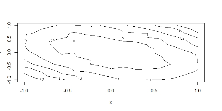
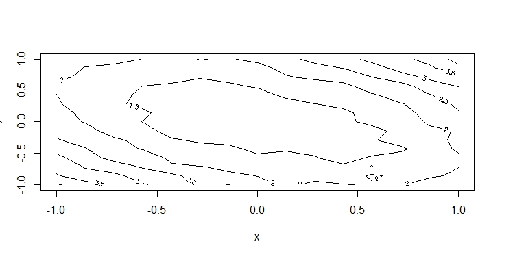
As it can be seen, we created three sets of x, y 'experiments', for three different levels of z. Practically, there is no limit on the sets we can include.The x,y contour plots for each z level are shown below:


open3d()
contour4D(x,y,W)
The result is then shown in an interactive 3D window and it can be plot and seen from various perspectives.

